Lately, the best part of my day has been figuring out the cool new things I can do in Google Sheets -- which, yes, definitely means I need to get out more, but also means I can share my favorite formulas with you.

![→ Access Now: Google Sheets Templates [Free Kit]](https://no-cache.hubspot.com/cta/default/53/e7cd3f82-cab9-4017-b019-ee3fc550e0b5.png)
How to Use Formulas for Google Sheets
- Double-click on the cell you want to enter the formula in. (If you want the formula for the entire row, this will probably be the first or second row in a column.)
- Type the equal (=) sign.
- Enter your formula. Depending on the data, Google Sheets might suggest a formula and/or range for you.
V-LOOKUP Google Sheets Formula
V-lookups, are by far, the most useful formula in your tool-kit when you’re working with large amounts of data. The V-lookup formula looks for a data point -- like, say, a blog post title or URL -- in one sheet, and returns a relevant piece of information for that data point -- like monthly views or conversion rate in another sheet.
For example, if I want to see how much traffic a specific set of blog posts got, I’ll export a list from Google Analytics, then put that list in another tab and use the V-LOOKUP function to pull views by URL into the first tab.
The only caveat: The data point must exist in both cells, and it must in the first column of the second sheet.
Formula:
=VLOOKUP(search_criterion, array, index, sort_order)
Let’s walk through an example, which should make this a bit easier to understand.
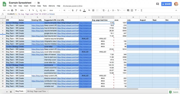
In the first sheet, I have a list of blog posts, including their titles, URLs and monthly traffic. In the second sheet, I have a report from Google Analytics with average page load time by URL. I want to see if there’s any correlation between page speed and performance.
An example:
=VLOOKUP(A2,’GA Avg. Load Time’’!$1:$1000,2,FALSE)
IFERROR Google Sheets Formula
Any time you’re using a formula where more than 10% of the return values lead to errors, your spreadsheet starts to look really messy (see the above screenshot!).
To give you an idea, maybe you have two columns: one for page views and another for CTA clicks. You want to see the highest-converting pages, so you create a third column for page views divided by CTA clicks (or =B2/C2).
About one-third of your pages, however, don’t have any CTAs -- so they haven’t gotten any clicks. This will show up as #VALUE! on your sheet, since you can’t divide by zero.
Using the IFERROR formula lets you replace the VALUE! Status with another value. I typically use a space (“ “) so the sheet is as clean as possible.
Here’s the formula:
=IFERROR(original_formula, value_if_error)
So for the above situation, my formula would be:
=IFERROR((B2/C2, “ “)
COUNTIF Google Sheets Formula
The COUNTIF formula tells you how many how many cells in a given range meet the criteria you’ve specified. With this up your sleeve, you’ll never have to manually count cells again.
Formula:
=COUNTIF(range, criterion)
Let’s say I’m curious how many blog posts received more than 1,000 views for this time period -- I’d enter:
=COUNTIF(C2:C500,“>1000”)
Or maybe I want to see how many blog posts were written by Caroline Forsey. If the author was in Column D, my formula would be:
=COUNTIF(D2:D500, “Caroline Forsey”)
LEN Google Sheets Function
Have you noticed Google Analytics cuts off the “http://” or “https://” from every URL? This posed a major issue for me when I wanted to combine data from HubSpot and GA -- the V-Lookup function wouldn’t work because the URLs weren’t identical (“https://blog.hubspot.com/marketing versus “blog.hubspot.com/marketing).
Luckily, there’s no need to manually change every URL. The LEN function lets you adapt the length of any string.
=LEFT(text,LEN(text)-n)
=RIGHT(text,LEN(text)-n)
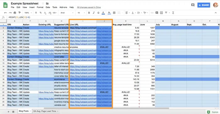
So, let’s say the full URL is in column I. To remove the “https://” string and make it identical to the URL in the Google Analytics tab, I’d use:
=RIGHT(I2, LEN(I2)-8)
If you wanted to remove the last characters in a cell, you’d simply change RIGHT to LEFT.
Array Formula for Google Sheets
Rarely do you need to apply a formula to a single cell -- you’re usually using it across a row or column. If you copy and paste a formula into a new cell, Google Sheets will automatically change it o reference the right cells; for example, if I enter =A2+B2 in cell C2, then drag the formula down to C3, the formula will become =A3+B3.
But there are a few drawbacks to this. First, if you’re working with a lot of data, having hundreds or thousands of formulas can make Google Sheets a lot slower. Second, if you change the formula -- maybe now you want to see =A2*B2 instead -- you have to make that change across every formula. Again, that’s time-consuming and requires a lot of processing power. And finally, the formula doesn’t automatically apply to new rows or columns.
An array formula solves these issues. It’s one formula, with one calculation, but the results are sorted into multiple rows or columns. Not only is this more efficient, but any changes will automatically apply to all your data.
ARRAYFORMULA(array_formula)
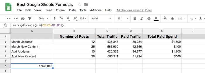
Let’s suppose I want to see how much non-paid traffic we’d gotten in March and April. That requires subtracting paid traffic from total (column D from column C) and then adding the totals together. Two separate formulas.
Or, I could use an array formula:
=ARRAYFORMULA(SUM(C2:C5-D2:D5)
The second part, SUM(C2:C5-D2:D5), should look somewhat familiar. It’s a traditional addition formula -- but it’s applied to a range (cells C2 through C5 and D2 through D5) instead of individual cells.
The first part, =ARRAYFORMULA, tells Google Sheets we’re applying this formula to a range.
I could also use an array formula to look at the non-paid traffic specifically from updates (not new content) in March and April.
Here’s what that would look like:
=ARRAYFORMULA(SUM(C2,C4-D2,D4))
IMPORTRANGE Google Sheets Formula
I use to spend a ton of time (and processing power) manually copying huge amounts of data from one spreadsheet to another. Then I learned about this handy formula, which imports data from a separate Google Sheets spreadsheet.
Suppose our resident historical optimization expert Braden Becker sent me a spreadsheet of the content he updated last month. I want to add that data to a master spreadsheet of all the content (both new and historically optimized) we published. I’d use this formula:
IMPORTRANGE(spreadsheet_url, range_string)
Which would look like:
IMPORTRANGE("https://docs.google.com/spreadsheets/d/abcd123abcd123", "Update Performance!A2:D100")
How to Split Text in Google Sheets
Splitting text can be incredibly useful when you’re dealing with different versions of the same URLs.
To give you an idea, let’s suppose I’ve created a spreadsheet with every URL that received at least 300 views in January and February. I want to compare the two months to see which blog posts got more views over time, fewer, or around the same.
The problem is, if I do a V-LOOKUP between the two tabs, Google Sheets won’t recognize these as the same URLs:
https://blog.hubspot.com/sales/songs-for-maximum-motivation (regular URL)
https://blog.hubspot.com/sales/songs-for-maximum-motivation?utm_medium=paid_EN&utm_content=songs-for-maximum-motivation&utm_source=getpocket.com&utm_campaign=PocketPromotion (tracking URL)
https://blog.hubspot.com/marketing/create-infographics-with-free-powerpoint-templates (regular URL)
https://blog.hubspot.com/marketing/create-infographics-with-free-powerpoint-templates?utm_medium=paid_EN&utm_content=create-infographics-with-free-powerpoint-templates&utm_source=getpocket.com&utm_campaign=PocketPromotion (tracking URL)
It would be awesome if I could get delete everything after the question mark in the tracking URLs so they matched the original ones.
That’s where the split text formula comes in.
=SPLIT(text, delimiter, [split_by_each], [remove_empty_text])
Text: The text you want to divide (can be a string of characters, such as https://blog.hubspot.com/marketing/create-infographics-with-free-powerpoint-templates?utm_medium=paid_EN&utm_content=create-infographics-with-free-powerpoint-templates&utm_source=getpocket.com&utm_campaign=PocketPromotion, or a cell, like A2)
Delimiter: The characters you want to split the text around.
Split_by_each: Google Sheets considers each character in the delimiter to be separate. That means if you split your text by “utm”, it will split everything around the characters “u”,”t”, and “m”. Include FALSE in your formula to turn this setting off.
In the example above, here’s the formula I’d use to split the first part of the URL from the UTM code:
=SPLIT(A2,“?”)
The first part is now in Column B, and the UTM code is in Column C. I can simply delete everything in Column C, and run the V-LOOKUP on the URLs in Column B.
Alternatively, you can use Google Sheet’s “Split text to columns” feature. Highlight the range of data you want to split, then select “Data” > “Split text to columns.”
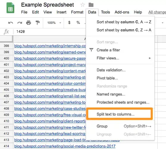
Now choose the character you want to delimit by: a colon, semicolon, period, space, or custom character. You can also opt for Google Sheets to figure out which character you want to split by (which it’s smart enough to do if your data is entered uniformly, e.g. every cell follows the same format) by choosing the first option, “detect automatically.”

I hope these Google Sheets formulas are helpful. If you have any other favorites, let me know on Twitter: @ajavuu.


![How to Highlight Duplicates in Google Sheets [Step-by-Step]](https://blog.hubspot.com/hubfs/highlight-duplicates-google-sheets_7.webp)
![How to Make a Histogram on Google Sheets [5 Steps]](https://blog.hubspot.com/hubfs/how%20to%20make%20a%20histogram%20on%20google%20sheets.jpg)