
Need to merge two sheets with similar data? Do simple math? Combine information in multiple cells? Excel can do it all.
In this post, I’ll review the best tips, tricks, and shortcuts for taking your Excel game to the next level. The best part? You don’t need advanced Excel knowledge.
.png)
50 Excel Hacks To Help You Master Excel
Tips to help you tackle Excel, including a guided template, GIF demonstrations, and a graph generator.
- 50 Excel Hacks
- A Guided Template
- GIF Visuals
- Excel Graph Generators
Download Free
All fields are required.
Form not available
What is Excel?
Microsoft Excel is powerful data visualization and analysis software. It uses spreadsheets to store, organize, and track data sets with formulas and functions.
Excel is used by marketers, accountants, data analysts, and other professionals. It's part of the Microsoft Office suite of products. Excel alternatives include Google Sheets and Numbers.
What is Excel used for?
Excel is used to store, analyze, and report on large amounts of data. It is often used by accounting teams for financial analysis but can be used by any professional to manage long and unwieldy datasets. Examples of Excel applications include balance sheets, budgets, or editorial calendars.
Excel is primarily used to create financial documents because of its strong computational powers. You’ll often find the software in accounting offices and teams because it allows accountants to automatically see sums, averages, and totals. With Excel, they can easily make sense of their business data.
While Excel is primarily known as an accounting tool, professionals in any field can use its features and formulas — especially marketers — because it’s valuable for tracking any type of data.
It removes the need to spend hours and hours counting cells or copying and pasting performance numbers. Excel typically has a shortcut or quick fix that speeds up the process.
There are several downloaded Excel templates you can use for your marketing needs. You can find some of them below.
While these templates will make using Excel less daunting, you still need to understand the basics.
Don’t worry. I’ve got you covered.
Excel Basics
There are a million and one things you could do with Excel. However, everything starts with opening an Excel Sheet or Workbook.
You can open an Excel Sheet by creating a new one or clicking on an existing one.
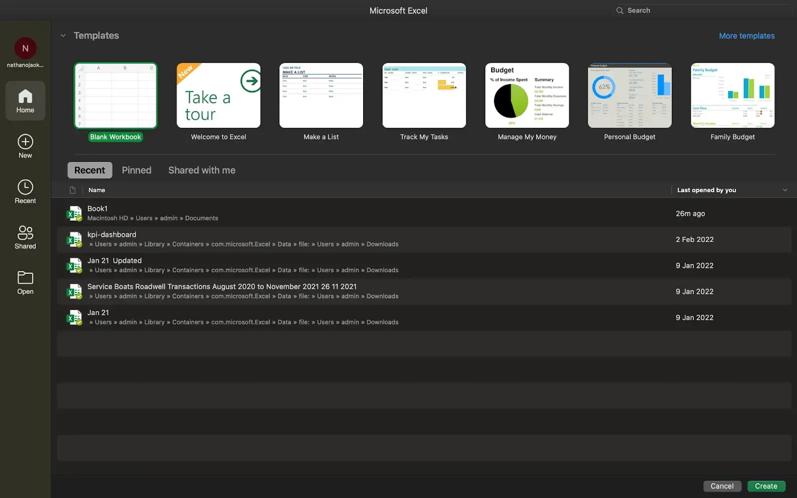
If you don’t have an existing worksheet, you can create one or choose from the many templates available in Excel.
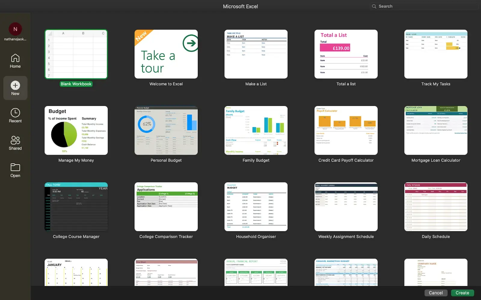
A blank Excel Sheet can be intimidating. However, it gets easier once you familiarize yourself with how the navigation works and what each different menu means.
There are usually seven tabs — Home, Insert, Draw, Page Layout, Formulas, Data, Review, and View — all with different functions that help you analyze and present your data.
I say “usually” because you can add the Developer tab if needed.
To add the Developer tab, click the vertical ellipsis icon at the top of your Excel Sheet. Click More Commands. Switch to the Ribbon view. There, you can choose the tabs you want to appear on your Excel Sheet.
Click the checkbox next to Developer to add it. After closing the menu, the Develop tab should appear on your Excel Sheet.
It’s okay if you don’t know everything about these menus yet. You’ll learn with practice.
As you’re just starting, here are some basic commands I suggest you become familiar with:
- Creating a new spreadsheet from scratch.
- Executing basic computations like adding, subtracting, multiplying, and dividing.
- Writing and formatting column text and titles.
- Using Excel's auto-fill features.
- Adding or deleting single columns, rows, and spreadsheets.
- Keeping column and row titles visible as you scroll past them in a spreadsheet so you know what data you're filling in as you move further down the document.
- Sorting your data in alphabetical order.
We’ll explore some of these functions in-depth later in the article.
To whet your appetite, let’s consider the auto-fill feature.
You likely already know this quick trick if you have any basic Excel knowledge. But to cover our bases, allow me to show you the glory of autofill.
Autofill lets you quickly fill adjacent cells with several data types, including values, series, and formulas.
There are multiple ways to deploy this feature, but the fill handle is among the easiest. Select the cells you want to be the source, locate the fill handle in the lower-right corner of the cell, and either drag the fill handle to cover the cells you want to fill or just double click:
Similarly, sorting is an important feature you'll want to know when organizing your data in Excel.
Sometimes, you may have a data list with no organization whatsoever. Maybe you exported a list of your marketing contacts or blog posts. Whatever the case, Excel’s sort feature will help you alphabetize any list.
Click on the data in the column you want to sort. Then click on the “Data” tab in your toolbar and look for the “Sort” option on the left.
If the “A” is on top of the “Z,” you can just click on that button once. If the “Z” is on top of the “A,” click on the button twice.
When the “A” is on top of the “Z,” your list will be sorted in alphabetical order. However, when the “Z” is on top of the “A,” your list will be sorted in reverse alphabetical order.
Next, let's explore more of the basics of Excel (along with advanced features).
50 Excel Hacks To Help You Master Excel
Tips to help you tackle Excel, including a guided template, GIF demonstrations, and a graph generator.
- 50 Excel Hacks
- A Guided Template
- GIF Visuals
- Excel Graph Generators
Download Free
All fields are required.
Form not available
How to Use Excel
To use Excel, you only need to input the data into the rows and columns. And then, you'll use formulas and functions to turn that data into insights.
We’ll go over the best formulas and functions you need to know. But first, let’s look at the types of documents you can create using the software. That way, you have an overarching understanding of how to use Excel daily.
Documents You Can Create in Excel
Not sure how you can actually use Excel in your team? Here is a list of documents you can create:
- Income statements. You can use an Excel spreadsheet to track a company’s sales activity and financial health.
- Balance sheets. Balance sheets are among the most common documents you can create with Excel. It gives you a holistic view of a company’s financial standing.
- Calendar. You can easily create a spreadsheet monthly calendar to track events or other date-sensitive information.
Here are some documents you can create specifically for marketers.
- Marketing budgets. Excel is a strong budget-keeping tool. You can create and track marketing budgets and spend using Excel.
Pro tip: If you don’t want to create a document from scratch, download our marketing budget templates for free.
- Marketing reports. If you don’t use a marketing tool like HubSpot’s Marketing Hub, you might need a dashboard with all your reports. Excel is an excellent tool for creating marketing reports.
Pro tip: Download free Excel marketing reporting templates here.
- Editorial calendars. You can create editorial calendars in Excel. The tab format makes tracking your content creation efforts for custom time ranges extremely easy.
Pro tip: Download a free editorial content calendar template here.
- Traffic and leads calculator. Because of its strong computational powers, Excel is an excellent tool for creating all sorts of calculators — including one for tracking leads and traffic.
Pro tip: Grab a free pre-made lead goal calculator to get a jump start.
The above is only a tiny sampling of the marketing and business documents you can create in Excel. We’ve created an extensive list of Excel templates you can use right now for marketing, invoicing, project management, budgeting, and more.

In the spirit of working more efficiently and avoiding tedious, manual work, here are a few Excel formulas and functions you’ll need to know.
Excel Formulas
It’s easy to get overwhelmed by the wide range of Excel formulas you can use to make sense of your data. If you’re just getting started using Excel, you can rely on the following formulas to carry out some complex functions without adding to the complexity of your learning path.
- Equal sign. Before creating any formula, you’ll need to write an equal sign (=) in the cell where you want the result to appear.
- Addition. To add the values of two or more cells, use the + sign. Example: =C5+D3.
- Subtraction. To subtract the values of two or more cells, use the - sign. Example: =C5-D3.
- Multiplication. To multiply the values of two or more cells, use the * sign. Example: =C5*D3.
- Division. To divide the values of two or more cells, use the / sign. Example: =C5/D3.
Here’s how the results of these formulas might look:
Putting all these together, you can create a formula that adds, subtracts, multiplies, and divides all in one cell. Example: =(C5-D3)/((A5+B6)*3).
For more complex formulas, you’ll need to use parentheses around the expressions to follow the PEMDAS order of operations. Keep in mind that you can use plain numbers in your formulas.
Excel Functions
Excel functions automate some of the tasks you would use in a typical formula. For instance, instead of using the + sign to add up a range of cells, you’d use the SUM function. Let’s look at a few more functions to help automate calculations and tasks.
- SUM. The SUM function automatically adds up a range of cells or numbers. To complete a sum, you would input the starting and final cells with a colon in between. Here’s what that looks like: SUM(Cell1:Cell2). Example: =SUM(C5:C30).
- AVERAGE. The AVERAGE function averages out the values of a range of cells. The syntax is the same as the SUM function: AVERAGE(Cell1:Cell2). Example: =AVERAGE(C5:C30).
- IF. The IF function allows you to return values based on a logical test. The syntax is as follows: IF(logical_test, value_if_true, [value_if_false]). Example: =IF(A2>B2,“Over Budget”,“OK”).
- VLOOKUP. The VLOOKUP function helps you search for anything on your sheet’s rows. The syntax is: VLOOKUP(lookup value, table array, column number, Approximate match (TRUE) or Exact match (FALSE)). Example: =VLOOKUP([@Attorney],tbl_Attorneys,4,FALSE).
- INDEX. The INDEX function returns a value from within a range. The syntax is INDEX(array, row_num, [column_num]).
- MATCH. The MATCH function looks for a certain item in a range of cells and returns the position of that item. It can be used in tandem with the INDEX function. The syntax is: MATCH(lookup_value, lookup_array, [match_type]).
- COUNTIF. The COUNTIF function returns the number of cells that meet certain criteria or have a certain value. The syntax is COUNTIF(range, criteria). Example: =COUNTIF(A2:A5,“London”).
Okay, ready to get into the nitty-gritty? Let’s get to it. (And to all the Harry Potter fans out there ... you’re welcome in advance.)
Excel Tips
- Use Pivot tables to recognize and make sense of data.
- Add more than one row or column.
- Use filters to simplify your data.
- Remove duplicate data points or sets.
- Transpose rows into columns.
- Split up text information between columns.
- Use these formulas for simple calculations.
- Get the average of numbers in your cells.
- Use conditional formatting to make cells automatically change color based on data.
- Use the IF Excel formula to automate certain Excel functions.
- Use dollar signs to keep one cell's formula the same regardless of where it moves.
- Use the VLOOKUP function to pull data from one area of a sheet to another.
- Use INDEX and MATCH formulas to pull data from horizontal columns.
- Use the COUNTIF function to make Excel count words or numbers in any range of cells.
- Combine cells using an ampersand(&).
- Add checkboxes.
- Hyperlink a cell to a website.
- Add drop-down menus.
- Use the format painter.
- Create tables with data.
- Use tables to conduct a what-if analysis.
- Make formulas easier to comprehend with named ranges.
- Group data to improve organization.
- Use Find & Select to streamline formatting.
- Protect your work.
- Create custom number formats.
- Customize the Excel ribbon.
- Improve visual presentation with text wrapping.
- Add emojis.
Note: Some of the GIFs and visuals are from a previous version of Excel. When applicable, the copy has been updated to provide instructions for users of both newer and older Excel versions.
1. Use Pivot tables to recognize and make sense of data.
Pivot tables are used to reorganize data in a spreadsheet. They won’t change the data you have, but they can sum up values and compare different information in your spreadsheet, depending on what you’d like them to do.
Let‘s consider an example. Let’s say I want to look at the number of people in each house at Hogwarts.
To create the Pivot Table, I go to Data > Pivot Table. If you’re using the most recent version of Excel, you’d go to Insert > Pivot Table. Excel will automatically populate your Pivot Table, but you can always change the order of the data. Then, you have four options to choose from.
- Report Filter. This allows you to look at specific rows in your dataset. For example, if I wanted to create a filter by house, I could choose to include only students in Gryffindor instead of all students.
- Column Labels. These would be your headers in the dataset.
- Row Labels. These could be your rows in the dataset. Both Row and Column labels can contain data from your columns (e.g., You can drag First Name to either the Row or Column label — it just depends on how you want to see the data.)
- Value. This section allows you to look at your data differently. Instead of just pulling in any numeric value, you can sum, count, average, max, min, count numbers, or do a few other manipulations with your data. In fact, by default, when you drag a field to Value, it always does a count.
Since I want to count the number of students in each house, I'll go to the Pivot table builder and drag the House column to the Row Labels and the Values. This will sum up the number of students associated with each house.
2. Add more than one row or column.
As you play around with your data, you might find you constantly need to add more rows and columns. Sometimes, you may need to add hundreds of rows. Doing this one by one would be super tedious. Luckily, there’s always an easier way.
To add multiple rows or columns in a spreadsheet, highlight the number of preexisting rows or columns you want to add. Then, right-click and select “Insert.”
In the example below, I want to add three rows. By highlighting three rows and then clicking insert, I'm able to add three blank rows to my spreadsheet quickly and easily.
3. Use filters to simplify your data.
When examining huge data sets, you’re sometimes only interested in data from rows that fit specific criteria.
That's where filters come in.
Filters allow you to pare down your data to look at only specific rows at one time. Excel allows you to add a filter to each column in your data, and from there, you can choose which cells you want to view at once.
Let’s take a look at the example below. Add a filter by clicking the Data tab and selecting “Filter.” Clicking the arrow next to the column headers, you’ll be able to choose whether you want your data to be organized in ascending or descending order, as well as which specific rows you want to show.
In my Harry Potter example, let's say I only want to see the students in Gryffindor. By selecting the Gryffindor filter, the other rows disappear.
Pro tip: Copy and paste the values in the spreadsheet when a Filter is on to do additional analysis in another spreadsheet.
4. Remove duplicate data points or sets.
Larger data sets tend to have duplicate content. For example, you may have a list of multiple contacts in a company and only want to see the number of companies you have. In situations like this, removing the duplicates comes in quite handy.
To remove your duplicates, highlight the row or column you want to remove duplicates of. Then, go to the Data tab and select “Remove Duplicates” (which is under the Tools subheader in the older version of Excel).
A pop-up will appear to confirm which data you want to work with. Select “Remove Duplicates,” and you're good to go.
You can also use this feature to remove an entire row based on a duplicate column value. So if you have three rows with Harry Potter's information and only need to see one, then you can select the whole dataset and remove duplicates based on email. Your resulting list will have unique names without any duplicates.
5. Transpose rows into columns.
When you have rows of data in your spreadsheet, you may want to transform the items in one of those rows into columns (or vice versa). It would take a lot of time to copy and paste each individual header. The transpose feature allows you to move your row data into columns or vice versa.
Start by highlighting the column that you want to transpose into rows. Right-click it, and then select “Copy.” Next, select the cells on your spreadsheet where you want your first row or column to begin. Right-click on the cell, and then select “Paste Special.”
A module will appear — at the bottom, you'll see an option to transpose. Check that box and select OK. Your column will now be transferred to a row or vice-versa.
Note: On newer versions of Excel, a drop-down will appear instead of a pop-up.
50 Excel Hacks To Help You Master Excel
Tips to help you tackle Excel, including a guided template, GIF demonstrations, and a graph generator.
- 50 Excel Hacks
- A Guided Template
- GIF Visuals
- Excel Graph Generators
Download Free
All fields are required.
Form not available
6. Split up text information between columns.
What if you want to split information in one cell into two different cells?
For example, maybe you want to pull someone’s company name through their email address. Or perhaps you want to separate someone's full name into a first and last name for your email marketing templates.
Thanks to Excel, both are possible. First, highlight the column that you want to split up. Next, go to the Data tab and select “Text to Columns.” A module will appear with additional information.
First, you need to select either “Delimited” or “Fixed Width.”
- “Delimited” means you want to break up the column based on characters such as commas, spaces, or tabs.
- “Fixed Width” means you want to select the exact location on all the columns that you want the split to occur.
In the example case below, let's select “Delimited” to separate the full name into first and last names.
Then, it’s time to choose the Delimiters. This could be a tab, semi-colon, comma, space, or something else. (“Something else” could be the “@” sign used in an email address, for example.)
In our example, let’s choose the space. Excel will then show you a preview of what your new columns will look like.
When you’re happy with the preview, press “Next.” This page will allow you to select Advanced Formats if you choose to. When you’re done, click “Finish.”
7. Use formulas for simple calculations.
In addition to doing pretty complex calculations, Excel can help you perform simple arithmetic, such as adding, subtracting, multiplying, or dividing any of your data.
- To add, use the + sign.
- To subtract, use the - sign.
- To multiply, use the * sign.
- To divide, use the / sign.
You can also use parentheses to ensure Excel performs specific calculations first. In the example below (10+10*10), the second and third 10 were multiplied together before adding the additional 10. However, if we made it (10+10)*10, the first and second 10 would be added together first.
8. Get the average of numbers in your cells.
If you want the average of a set of numbers, you can use the formula =AVERAGE(Cell1:Cell2). If you want to sum up a column of numbers, use the formula =SUM(Cell1:Cell2).
9. Use conditional formatting to make cells automatically change color based on data.
Conditional formatting allows you to change a cell's color based on the information within the cell.
For example, if you want to flag specific numbers above average or in the top 10% of the data in your spreadsheet, color code commonalities between different rows in Excel, or something else, you can do that.
This will help you quickly see information that is important to you.
To get started, highlight the group of cells you want to use conditional formatting on. Then, choose “Conditional Formatting” from the Home menu and select your logic from the dropdown. (You can also create your own rule if you want something different.)
A window will pop up that prompts you to provide more information about your formatting rule. Select “OK” when you're done, and you should see your results automatically appear.
10. Use the IF Excel formula to automate certain Excel functions.
Sometimes, we don't want to count the number of times a value appears. Instead, we want to input different information into a cell if there is a corresponding cell with that information.
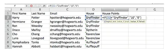
For example, in the situation below, I want to award ten points to everyone who belongs in the Gryffindor house. Instead of manually typing in 10‘s next to each Gryffindor student’s name, I can use the IF Excel formula to say that if the student is in Gryffindor, then they should get ten points.
The formula is: IF(logical_test, value_if_true, [value_if_false])
Example Shown Below: =IF(D2=“Gryffindor”,“10”,“0”)
In general terms, the formula would be IF(Logical Test, value of true, value of false). Let's dig into each of these variables.
- Logical_Test. The logical test is the “IF” part of the statement. In this case, the logic is D2=“Gryffindor” because we want to make sure that the cell corresponding with the student says “Gryffindor.” Make sure to put Gryffindor in quotation marks here.
- Value_if_True. This is what we want the cell to show if the value is true. In this case, we want the cell to show “10” to indicate that the student was awarded the 10 points.
- Value_if_False. This is what we want the cell to show if the value is false. In this case, for any student not in Gryffindor, we want the cell to show “0”.
Note: Only use quotation marks if you want the result to be text instead of a number.
Note: In the example above, I awarded 10 points to everyone in Gryffindor. If I later wanted to sum the total number of points, I wouldn’t be able to because the 10’s are in quotes, thus making them text and not a number that Excel can sum.
The real power of the IF function comes when you string multiple IF statements together or nest them. This allows you to set multiple conditions, get more specific results, and ultimately organize your data into more manageable chunks.
Ranges are one way to segment your data for better analysis. For example, you can categorize data into values less than 10, 11 to 50, or 51 to 100. Here's how that looks in practice:
=IF(B3<11,“10 or less”,IF(B3<51,“11 to 50”,IF(B3<100,“51 to 100”)))
It can take some trial and error, but once you have the hang of it, IF formulas will become your new Excel best friend.
11. Use dollar signs to keep one cell's formula the same regardless of where it moves.
Have you ever seen a dollar sign in an Excel formula? When used in a formula, it doesn't represent an American dollar; instead, it ensures that the exact column and row are held the same even if you copy the same formula in adjacent rows.
You see, a cell reference — when you refer to cell A5 from cell C5, for example — is relative by default. In that case, you’re actually referring to a cell that’s five columns to the left (C minus A) and in the same row (5).
This is called a relative formula. When you copy a relative formula from one cell to another, it’ll adjust the values in the formula based on where it’s moved.
But sometimes, we want those values to stay the same no matter whether they're moved around or not — and we can do that by turning the formula into an absolute formula.
To change the relative formula (=A5+C5) into an absolute formula, we'd precede the row and column values by dollar signs like this: (=$A$5+$C$5). (Learn more on Microsoft Office's support page here.)
12. Use the VLOOKUP function to pull data from one area of a sheet to another.
Have you ever had two sets of data on two different spreadsheets that you want to combine into a single spreadsheet?
For example, you might have a list of people’s names next to their email addresses in one spreadsheet and a list of those same people’s email addresses next to their company names in the other — but you want the names, email addresses, and company names of those people to appear in one place.
I have to combine data sets like this a lot — and when I do, the VLOOKUP is my go-to formula.
Before you use the formula, though, be absolutely sure that you have at least one column that appears identically in both places. Scour your data sets to ensure the column of data you're using to combine your information is the same, including no extra spaces.
The formula: =VLOOKUP(lookup value, table array, column number, Approximate match (TRUE) or Exact match (FALSE))
The formula with variables from our example below: =VLOOKUP(C2,Sheet2!A:B,2,FALSE)
In this formula, there are several variables. The following is true when you want to combine information in Sheet 1 and Sheet 2 into Sheet 1.
- Lookup Value. This is the identical value you have in both spreadsheets. Choose the first value in your first spreadsheet. In the following example, this means the first email address on the list or cell 2 (C2).
- Table Array. The table array is the range of columns on Sheet 2 you‘re going to pull your data from, including the column of data identical to your lookup value (in our example, email addresses) in Sheet 1, as well as the column of data you’re trying to copy to Sheet 1. In our example, this is “Sheet2!A:B.” “A” means Column A in Sheet 2, which is the column in Sheet 2 where the data identical to our lookup value (email) in Sheet 1 is listed. The “B” means Column B, which contains the information only available in Sheet 2 that you want to translate to Sheet 1.
- Column Number. This tells Excel which column the new data you want to copy to Sheet 1 is located in. In our example, this would be the column that “House” is located in. “House” is the second column in our range of columns (table array), so our column number is 2. [Note: Your range can be more than two columns. For example, if there are three columns on Sheet 2 — Email, Age, and House — and you still want to bring House onto Sheet 1, you can still use a VLOOKUP. You just need to change the “2” to a “3” so it pulls back the value in the third column: =VLOOKUP(C2:Sheet2!A:C,3,false).]
- Approximate Match (TRUE) or Exact Match (FALSE). Use FALSE to ensure you pull in only exact value matches. If you use TRUE, the function will pull in approximate matches.
In the example below, Sheet 1 and Sheet 2 contain lists describing different information about the same people, and the common thread between the two is their email addresses. Let's say we want to combine both datasets so that all the house information from Sheet 2 translates over to Sheet 1.
So when we type in the formula =VLOOKUP(C2,Sheet2!A:B,2,FALSE), we bring all the house data into Sheet 1.
Remember that VLOOKUP will only pull back values from the second sheet to the right of the column containing your identical data. This can lead to some limitations, which is why some people prefer to use the INDEX and MATCH functions instead.
50 Excel Hacks To Help You Master Excel
Tips to help you tackle Excel, including a guided template, GIF demonstrations, and a graph generator.
- 50 Excel Hacks
- A Guided Template
- GIF Visuals
- Excel Graph Generators
Download Free
All fields are required.
Form not available
13. Use INDEX and MATCH formulas to pull data from horizontal columns.
Like VLOOKUP, the INDEX and MATCH functions pull data from another dataset into one central location. Here are the main differences:
- VLOOKUP is a much simpler formula. If you're working with large data sets requiring thousands of lookups, using the INDEX and MATCH functions will significantly decrease load time in Excel.
- The INDEX and MATCH formulas work right-to-left, whereas VLOOKUP formulas only work as a left-to-right lookup. In other words, if you need to do a lookup with a lookup column to the right of the results column, then you'd have to rearrange those columns to do a VLOOKUP. This can be tedious with large datasets and/or lead to errors.
So if I want to combine information in Sheet 1 and Sheet 2 onto Sheet 1, but the column values in Sheets 1 and 2 aren‘t the same, then to do a VLOOKUP, I would need to switch around my columns. In this case, I’d choose to do an INDEX and MATCH instead.
Let’s look at an example. Let’s say Sheet 1 contains a list of people’s names and their Hogwarts email addresses, and Sheet 2 contains a list of people’s email addresses and each student's Patronus. (For non-Harry Potter fans, every witch or wizard has an animal guardian called a “Patronus” associated with them.)
The information that lives in both sheets is the column containing email addresses, but this email address column is in different column numbers on each sheet. I‘d use the INDEX and MATCH formulas instead of VLOOKUP so I wouldn’t have to switch any columns around.
So what’s the formula, then? The formula is actually the MATCH formula nested inside the INDEX formula. You’ll see I differentiated the MATCH formula using a different color here.
The formula: =INDEX(table array, MATCH formula)
This becomes: =INDEX(table array, MATCH (lookup_value, lookup_array))
The formula with variables from our example below: =INDEX(Sheet2!A:A,(MATCH(Sheet1!C:C,Sheet2!C:C,0)))
Here are the variables:
- Table Array. The range of columns on Sheet 2 containing the new data you want to bring to Sheet 1. In our example, “A” means Column A, which contains the “Patronus” information for each person.
- Lookup Value. This is the column in Sheet 1 that contains identical values in both spreadsheets. In the example that follows, this means the “email” column on Sheet 1, which is Column C. So: Sheet1!C:C.
- Lookup Array. This is the column in Sheet 2 that contains identical values in both spreadsheets. In the example that follows, this refers to the “email” column on Sheet 2, which happens to also be Column C. So: Sheet2!C:C.
Once you have your variables straight, type in the INDEX and MATCH formulas in the top-most cell of the blank Patronus column on Sheet 1, where you want the combined information to live.
14. Use the COUNTIF function to make Excel count words or numbers in any range of cells.
Instead of manually counting how often a specific value or number appears, let Excel do the work for you. With the COUNTIF function, Excel can count the number of times a word or number appears in any range of cells.
For example, let's say I want to count the number of times the word “Gryffindor” appears in my data set.
The formula: =COUNTIF(range, criteria)
The formula with variables from our example below: =COUNTIF(D:D,“Gryffindor”)
In this formula, there are several variables:
- Range. The range that we want the formula to cover. In this case, since we're only focusing on one column, we use “D:D” to indicate that the first and last columns are both D. If I were looking at columns C and D, I would use “C:D.”
- Criteria. Whatever number or piece of text you want Excel to count. Only use quotation marks if you want the result to be text instead of a number. In our example, the criteria is “Gryffindor.”
Simply typing in the COUNTIF formula in any cell and pressing “Enter” will show me how many times the word “Gryffindor” appears in the dataset.
15. Combine cells using an ampersand (&).
Databases tend to split out data to make it as exact as possible.
For example, instead of having a column that shows a person‘s full name, a database might have the data as a first name and then a last name in separate columns.
Or, it may have a person’s location separated by city, state, and zip code. In Excel, you can combine cells with different data into one cell using the “&” sign in your function.
The formula with variables from our example below: =A2&“ ”&B2
Let‘s go through the formula together using an example. Pretend we want to combine first and last names into full names in a single column.
To do this, we’d first put our cursor in the blank cell where we want the full name to appear. Next, we'd highlight one cell that contains a first name, type in an “&” sign, and then highlight a cell with the corresponding last name.
But you‘re not finished — if all you type in is =A2&B2, there will not be a space between the person’s first and last names. To add that necessary space, use the function =A2&“ ”&B2. The quotation marks around the space tell Excel to put a space between the first and last names.
To make this true for multiple rows, drag the corner of that first cell downward, as shown in the example.
16. Add checkboxes.
If you’re using an Excel sheet to track customer data and want to oversee something that isn’t quantifiable, you could insert checkboxes into a column.
For example, if you’re using an Excel sheet to manage your sales prospects and want to track whether you called them in the last quarter, you could have a “Called this quarter?” column and check off the cells in it when you’ve called the respective client.
Here's how to do it.
Highlight a cell to which you'd like to add checkboxes to your spreadsheet. Then, click Developer and then Checkbox.
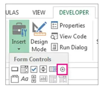
Drag or copy the checkbox to the cells where you want them to appear.
17. Hyperlink a cell to a website.
If you‘re using your sheet to track social media or website metrics, it can be helpful to have a reference column with the links each row is tracking.
If you add a URL directly into Excel, it should automatically be clickable. But, if you have to hyperlink words like a page title or the headline of a post you’re tracking, here's how.
Highlight the words you want to hyperlink, then press Shift K. A box will pop up, allowing you to place the hyperlink URL. Copy and paste the URL into this box and hit or click Enter.
If the key shortcut isn't working for any reason, you can also do this manually. Highlight the cell, right-click, and choose Hyperlink from the drop-down menu.
18. Add drop-down menus.
Sometimes, you’ll use your spreadsheet to track processes or other qualitative things. Rather than writing words into your sheet repetitively, such as “Yes,” “No,” “Customer Stage,” “Sales Lead,” or “Prospect,” you can use dropdown menus to quickly mark descriptive things about your contacts or whatever you’re tracking.
Here's how to add drop-downs to your cells.
Highlight the cells you want the drop-downs to be in, then click the Data menu in the top navigation and press Validation.
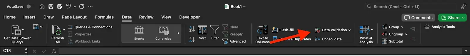
From there, a Data Validation Settings box will open. Look at the Allow options, then click Lists and select Drop-down List. Check the In-Cell dropdown button, then press OK.
19. Use the format painter.
As you’ve probably noticed, Excel has many features to make crunching numbers and analyzing your data quick and easy. But if you've ever spent some time formatting a sheet to your liking, you know it can get a bit tedious.
Don’t waste time repeating the same formatting commands over and over again.
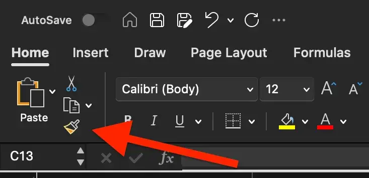
Use the format painter to easily copy the formatting from one area of the worksheet to another. To do so, choose the cell you’d like to replicate, then select the format painter option (paintbrush icon) from the top toolbar.
20. Create tables with data.
Converting your data into a table makes it visually appealing and provides improved data management and analysis capabilities.
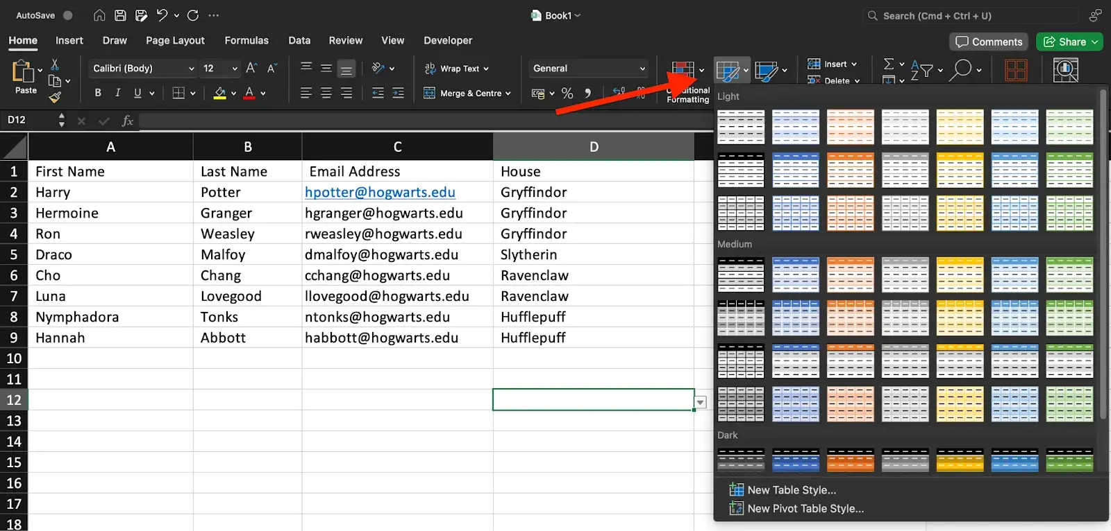
To get started, you’ll need to select the range of cells that you want to convert into a table. Then, go to the Home tab in the Excel ribbon. In the Styles group, click the Format as Table button — it looks like a grid of cells. Then, choose a table style from the available options or customize a table if desired.
In the Create Table dialog box, make sure the range you selected is correct. If Excel does not automatically detect the range correctly, you can adjust it manually.
If your table has headers (column names), ensure that the “My table has headers” option is checked. This allows Excel to treat the first row as the header row.
Once everything is ready, click the OK button, and Excel will convert your selected data into a table.
After your data is converted into a table, you'll notice some additional features and functionalities become available:
- The table is automatically assigned a name, such as “Table1” or “Table2,” which you can modify if needed.
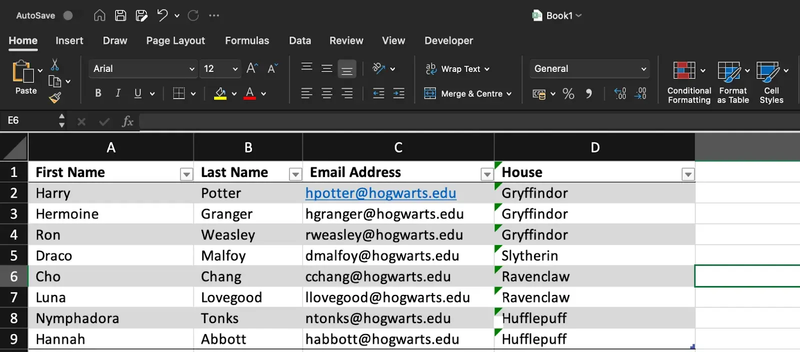
- Filter drop-down arrows appear in the header row, allowing you to filter data within the table easily.
- The table is formatted with alternating row colors, making it visually appealing.
- Total rows are automatically added at the bottom of each column, allowing you to perform calculations like sum, average, etc., for the data in that column.
50 Excel Hacks To Help You Master Excel
Tips to help you tackle Excel, including a guided template, GIF demonstrations, and a graph generator.
- 50 Excel Hacks
- A Guided Template
- GIF Visuals
- Excel Graph Generators
Download Free
All fields are required.
Form not available
21. Use tables to conduct a what-if analysis.
In addition to making your data more organized, tables can help you conduct what-if analyses. This allows you to test various combinations of input values and observe the resulting outcomes.
What-if analysis can be beneficial in decision-making, planning, forecasting, financial modeling, sensitivity analysis, resource planning, and more.
To get started, you’ll need to set up your worksheet with the necessary formulas and variables you want to analyze. Then, determine the input values that you want to vary. Typically, you will choose one or two input variables.
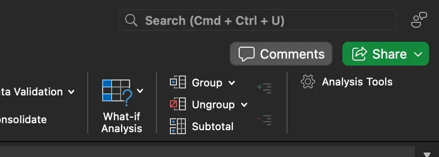
Select the cell where you want to display the results of your what-if analysis. Then, click the What-If Analysis button in the Data tab. From the dropdown menu, select Data Table.
In the Table Input dialog box, enter the input values that you want to test for each variable. If you have one variable, enter the different input values in a column or row. If you have two variables, enter the combinations in a table format.
Select the cells in the table area corresponding to the formula cell you want to analyze. This is the cell that will display the results for each combination of input values.
Click OK to generate the data table. Excel will calculate the formula for each combination of input values and display the results in the selected cells. The data table acts as a grid, showing the various scenarios and their corresponding outcomes.
Once your table is created, you can use it to identify trends, patterns, or specific values of interest. Play around with the input values and see how it may affect the final results.
22. Make formulas easier to comprehend with named ranges.
Instead of referring to a range of cells by its coordinates (e.g., A1:B10), you can assign a name to it. This makes formulas more readable and easier to manage.
To get started, select the cell or range you want to name. Go to the Formulas tab in the Excel ribbon and click on the Define Name button in the Defined Names group.
In the New Name dialog box, enter a name for the selected cell or range in the Name field. Make sure the name is descriptive and easy to remember.
By default, Excel assigns the selected cell or range's reference to the Refers to field in the dialog box. If needed, you can modify the reference to include additional cells or adjust the range.
Click the OK button to save the named range. Once you've named a range, you can use it in your formulas by simply typing the name instead of the cell reference. For example, if you named cell A1 as “Revenue,” you could use =Revenue instead of =A1 in your formulas.
Using named ranges offers several benefits:
- Improved formula readability. Named ranges make formulas more straightforward to understand and navigate, especially in complex calculations or large datasets.
- Flexibility for range adjustments. If your dataset changes, you can easily modify the range assigned to a named range without updating each formula that references it.
- Enhanced collaboration. Named ranges make it easier to collaborate with others, as they can understand the purpose of a named range and use it in their own calculations.
- Simplified data analysis. When using named ranges, you can create more intuitive data analysis by referring to named ranges in functions like SUM, AVERAGE, COUNTIF, etc.
To manage named ranges, go to the Formulas tab and click on the Name Manager button in the Defined Names group. The Name Manager offers functionalities to modify, delete, or review existing named ranges.
23. Group data to improve organization.
Grouping data in Excel allows you to organize, analyze, and present information more effectively, making it easier to identify patterns, trends, and insights within your data. For instance, if you have a list of leads generated, you can group the data by month to create a monthly performance report.
Grouping data especially makes it easier to navigate and work with large data sets. It helps in organization and reduces clutter by collapsing the groups that are not immediately needed.
To group data in Excel, select the range of cells or columns that you want to group. Make sure the data is sorted properly if needed.
On the Data tab in the Excel ribbon, click on the Group button. It is usually found in the Outline or Data Tools group.
You can specify the grouping levels by choosing options like Rows or Columns. For example, you can select Months if you want to group data by month.
You can also set additional options, such as Summary rows below details, or collapse the outline to the summary levels. These options affect how the grouped data is displayed.
Once you have the options you want selected, click on the OK button, and Excel will group the selected data based on your settings.
After your data is grouped, you will see a plus (+) or minus (-) button next to the grouped rows or columns. Clicking on the plus button expands the group to show the individual records, and clicking on the minus button collapses the group to hide the details.
24. Use Find & Select to streamline formatting.
Why format and clean up your spreadsheet manually when you can do it in just a few clicks? Using the Find & Select tool can help you maintain document accuracy and consistency.
To get started, open the Excel worksheet that contains the data you want to search. Press the Ctrl + F keys on your keyboard or go to the Home tab and click on the Find & Select drop-down menu. Then, select Find from the menu. The Find and Replace dialog box will open.

In the Find field, enter the specific data you want to find. Optionally, you can narrow your search to particular cells, rows, columns, or formulas by choosing the appropriate options in the dialog box.
Click on the Find Next button to search for the first occurrence of the data. Excel will highlight the cell containing the data.
To replace the found data with new information, click the Replace button in the dialog box. This will replace the highlighted occurrence with the data you enter in the Replace field.
To replace all occurrences of the data at once, click on the Replace All button. You can close the dialog box once you have finished finding and replacing what you want.
Note: Be cautious when using the Replace All feature, as it replaces all occurrences without confirmation. It is always a good practice to review each replacement carefully before using the Replace All option.
25. Protect your work.
Protecting your work in Excel is essential for data security, maintaining data integrity, preserving intellectual property, and complying with legal or regulatory requirements. It allows you to control who can access and modify your work, minimizing risks and maintaining the quality and confidentiality of your data.
Here are a couple of ways you can protect your work:
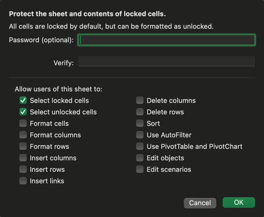
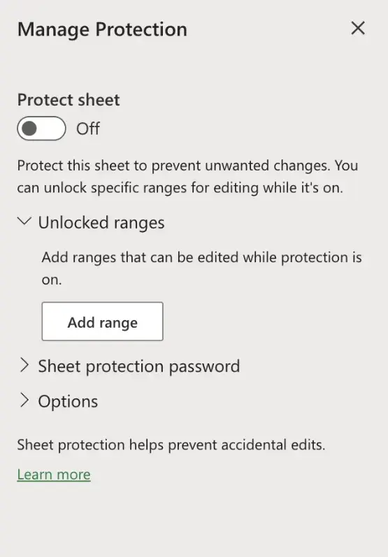
Protect a Worksheet
- Open your Excel worksheet and navigate to the Review tab.
- Click Protect Sheet.
- A Manage Protection dialog box will appear. There, you can select whether or not you want to protect the sheet. Set a password if desired and choose the options you wish to apply, such as preventing users from making changes to cells, formatting, inserting/deleting columns or rows, etc.
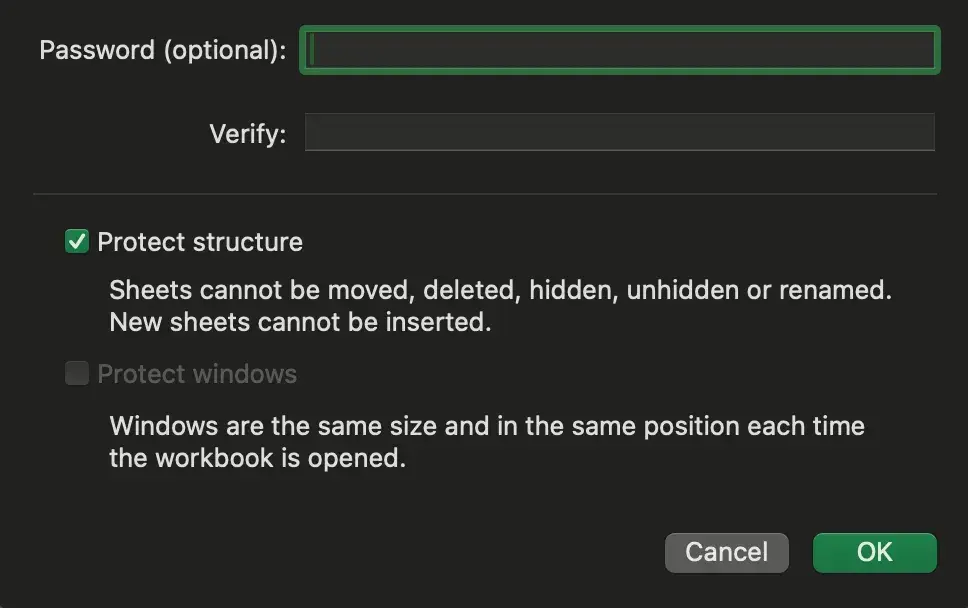
Protecting a Workbook
This follows a process similar to protecting a worksheet. The Protect Workbook selection is next to the Protect Worksheet selection.
After clicking Protect Workbook, choose your password.
Taking these extra steps ensures your work is protected. Just make sure to keep your passwords safe and secure.
26. Create custom number formats.
To display data in unique ways, use custom number formats. Doing this can help with data presentation, data clarity, consistency, localization, and masking of sensitive data.
To get started, select the cell or range of cells you want to format. Then, click the menu above the percentage sign under the Home tab.
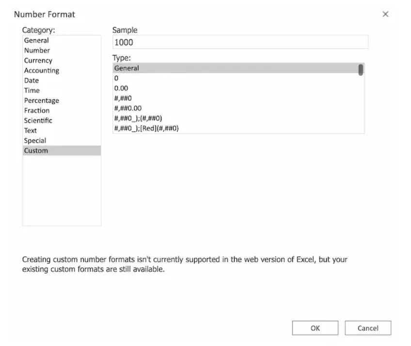
Select More Number Formats from the dropdown. Select Custom.
In the Type field, you can enter a custom number format code to define your desired format. Here are some examples of custom number formats:
- To display numbers with a specific number of decimal places, use the 0 or # symbol to represent a digit and a zero or hashtag without a decimal point to represent optional digits. For example, 0.00 will display two decimal places, 0.### will display up to three decimal places, and ### will display no decimal places.
- To display a specific text or character alongside numbers, use the @ symbol. For example, $0 will display a dollar sign before the number.
- To display percentages, use the % symbol. For example, 0% will display the number as a percentage.
- To create custom date or time formats, use codes such as dd for day, mm for month, yy for two-digit year, hh for hours, mm for minutes, and ss for seconds. For example, dd/mm/yyyy will display the date in the day/month/year format.
As you enter your custom number format in the Type field, you will see a Sample section showing how the format will be applied. Click OK to apply the custom number format to the selected cells.
27. Customize the Excel ribbon.
Although the Excel ribbon already contains various tools for executing common functions and commands, you can customize it to fit your specific needs and preferences.
This can help streamline your workflow and make commonly used commands more easily accessible. It also allows you to remove unnecessary elements that you don’t use, making it easier to navigate and find the tools you need.

To make customizations, start by right-clicking on an empty ribbon area and selecting Customize the Ribbon. In the Excel Options window that appears, you'll see two sections. The left section displays the tabs currently visible in the ribbon, while the right section displays the tabs you can add.
To customize the ribbon, you have several options:
- To add a new tab, click on New Tab in the right section and give it a name.
- To add a group within an existing tab, select the tab in the left section, click New Group in the right section, and name it.
- To add commands to a group, select the group in the right section, choose commands from the left section, and click Add. You can also customize the order of the commands using the Up and Down buttons.
You can also remove tabs, groups, or commands from the ribbon. Select the item you want to remove in the left section and click Remove.
To change the order of tabs and groups, select the item in the left section and use the Up and Down buttons to rearrange them.
Click OK in the Excel Options window to save your changes and apply the customized ribbon.
To extend Excel’s functionality even further, you can customize the ribbon with additional applications by clicking on the Add-ins button in the Home tab.
Note: Customizing the ribbon is specific to your Excel installation and won‘t affect other users’ ribbons.
28. Improve visual presentation with text wrapping.

Even though spreadsheets aren’t always the most exciting things to look at, you can still take the time to make them easier to read by wrapping text.
Doing this lets you display multiple lines of text within a single cell. It's convenient when you need to include line breaks or break up paragraphs of information within a cell without increasing the row height.
Select the cell(s) with the text you want to wrap. Navigate to the toolbar at the top of the Excel window and locate the Wrap Text button (an icon with an angled arrow). It is typically found in the Alignment section. Then, click on Wrap Text.
29. Add emojis.
Give your spreadsheets a little personal touch by adding emojis.
To start, click on the cell where you want to insert an emoji. Then, open the emoji keyboard. This step may vary based on your operating system.
- Windows. Use the keyboard shortcut Win + . or Win + ; to open the emoji keyboard.
- macOS. Use the keyboard shortcut Ctrl + Cmd + Space to access the emoji keyboard.
Browse the available emojis and click on the one you want to insert. The selected emoji should now appear in the selected cell.

Emojis may appear small by default in Excel cells. To make them larger and improve visibility, you can adjust the cell size by dragging the row height and column width accordingly.
You can also copy emojis from external sources on the web or other applications and paste them directly into Excel cells.
Note: The ability to use emojis in Excel depends on the version of Excel and the device you are using. Some older versions or platforms may not support emojis or display them correctly. Therefore, it's essential to ensure compatibility with the Excel version and platform you are working with.
Excel Keyboard Shortcuts
Creating reports in Excel is time-consuming enough. How can we spend less time navigating, formatting, and selecting items in our spreadsheet?
I'm glad you asked. There are a ton of Excel shortcuts out there, including some of our favorites listed below.
Create a New Workbook
PC: Ctrl-N | Mac: Command-N
Select Entire Row
PC: Shift-Space | Mac: Shift-Space
Select Entire Column
PC: Ctrl-Space | Mac: Control-Space
Select the Rest of the Column
PC: Ctrl-Shift-Down/Up | Mac: Command-Shift-Down/Up
Select the Rest of the Row
PC: Ctrl-Shift-Right/Left | Mac: Command-Shift-Right/Left
Add Hyperlink
PC: Ctrl-K | Mac: Command-K
Open Format Cells Window
PC: Ctrl-1 | Mac: Command-1
Autosum Selected Cells
PC: Alt-= | Mac: Command-Shift-T
Other Excel Help Resources
- How to Make a Chart or Graph in Excel [With Video Tutorial]
- Totally Free Microsoft Excel Templates That Make Marketing Easier
- How to Learn Excel Online: Free and Paid Resources for Excel Training
Use Excel to Automate Processes in Your Team
Even if you’re not an accountant, you can still use Excel to automate tasks and processes in your team. With the tips and tricks we shared in this post, you’ll be sure to use Excel to its fullest extent and get the most out of the software to grow your business.
Editor's Note: This post was originally published in August 2017 but has been updated for comprehensiveness.
50 Excel Hacks To Help You Master Excel
Tips to help you tackle Excel, including a guided template, GIF demonstrations, and a graph generator.
- 50 Excel Hacks
- A Guided Template
- GIF Visuals
- Excel Graph Generators
Download Free
All fields are required.
Form not available
Excel


![How to Use VLOOKUP Function in Microsoft Excel [+ Video Tutorial]](https://53.fs1.hubspotusercontent-na1.net/hubfs/53/VLOOKUP-hero.webp)